7

This chapter lays out the basic logic and process of hypothesis testing. We will perform z tests, which use the z score formula from Chapter 6 and data from a sample mean to make an inference about a population.

Social Justice and Hypothesis Testing
Hypothesis testing allows us to move from description to action — it is the process that helps us decide whether patterns we see in data are likely due to chance or reflect real differences in the world. In social justice research, this means testing questions like: Are students of color disciplined more often than white students? Do women earn less than men, even when doing the same work? By setting up null and alternative hypotheses and using probability, we can examine whether inequalities are simply random variation or evidence of systemic bias.

We have learned to calculate means, medians and modes as well as variance and standard deviations to describe data.  Now we are moving on to make predictions and inferences about data.  This involves developing a null and research hypothesis and using probabilities to determine if we can predict an outcome.  For example, if we want to know the likelihood that that a person of color will be pulled over by the police compared to a White person, we can develop a research and null hypothesis to test that prediction.  To do this we need to collect data on the amount of times a person of color is stopped by police as well as the number of times a White person is stopped.  We might predict that it is much more likely to be pulled over if you are not White.  We can set up hypotheses to test that prediction.

The Null Hypothesis

The hypothesis that an apparent effect is due to chance is called the null hypothesis, written H0 (“H-naught”). In the Physicians’ Reactions example, the null hypothesis is that in the population of physicians, the mean time expected to be spent with obese patients is equal to the mean time expected to be spent with average-weight patients. This null hypothesis can be written as:

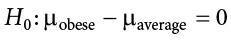
 Another simpler way to state this null hypothesis would be:

Ho: obese time = average time 

Essentially, both Ho’s are saying there is no difference between the time spent with obese patients and average weight patients.

Keep in mind that the null hypothesis is typically the opposite of the researcher’s hypothesis. In the Physicians’ Reactions study, the researchers hypothesized that physicians would expect to spend less time with obese patients. The null hypothesis that the two types of patients are treated identically is put forward with the hope that it can be discredited and therefore rejected. If the null hypothesis were true, a difference as large as or larger than the sample difference of 6.7 minutes would be very unlikely to occur. Therefore, the researchers rejected the null hypothesis of no difference and concluded that in the population, physicians intend to spend less time with obese patients.

Example:
Suppose we want to test whether women faculty are promoted at the same rate as men. The null hypothesis (H₀) would state there is no difference in promotion rates between men and women. This becomes our baseline assumption until we see strong evidence otherwise. The research hypothesis (Hₐ) would predict a difference — for example, that women are promoted less often.

In general, the null hypothesis is the idea that nothing is going on: there is no effect of our treatment, no relationship between our variables, and no difference in our sample mean from what we expected about the population mean. This is always our baseline starting assumption, and it is what we seek to reject. If we are trying to treat depression, we want to find a difference in average symptoms between our treatment and control groups.  However, until we have evidence against it, we must use the null hypothesis as our starting point.

The Alternative  (also called the Research) Hypothesis

If the null hypothesis is rejected, then we will need some other explanation, which we call the alternative hypothesis, HA or H1 or Hr. The alternative hypothesis is simply the reverse of the null hypothesis, and there are three options, depending on where we expect the difference to lie. Thus, our alternative hypothesis is the mathematical way of stating our research question. If we expect our obtained sample mean to be above or below the null hypothesis value, which we call a directional hypothesis, then our alternative hypothesis takes the form

based on the research question itself. We should only use a directional hypothesis if we have good reason, based on prior observations or research, to suspect a particular direction. When we do not know the direction, such as when we are entering a new area of research, we use a non-directional alternative:

Social Justice Example

If we are investigating police stops, the null might be that Black and white drivers are stopped at the same rate. The research hypothesis would be that Black drivers are stopped more frequently. Whether we make this directional (greater than) or non-directional (simply “different”) depends on prior evidence and theory.

We will set different criteria for rejecting the null hypothesis based on the directionality (greater than, less than, or not equal to) of the alternative. To understand why, we need to see where our criteria come from and how they relate to z scores and distributions.

Critical Values, p Values, and Significance Level

A low probability value casts doubt on the null hypothesis. How low must the probability value be in order to conclude that the null hypothesis is false? Although there is clearly no right or wrong answer to this question, it is conventional to conclude the null hypothesis is false if the probability value is less than .05. More conservative researchers conclude the null hypothesis is false only if the probability value is less than .01. When a researcher concludes that the null hypothesis is false, the researcher is said to have rejected the null hypothesis. The probability value below which the null hypothesis is rejected is called the level or simply (“alpha”). It is also called the significance level. If is not explicitly specified, assume that a = .05.

The significance level is a threshold we set before collecting data in order to determine whether or not we should reject the null hypothesis. We set this value beforehand to avoid biasing ourselves by viewing our results and then determining what criteria we should use. If our data produce values where the significance level, a=.05 or less , then we have sufficient evidence to reject the null hypothesis; if not and the probability or a is above .05, we fail to reject the null (we never “accept” the null).

Example:
Consider wage gaps. If our sample shows women earning less than men, we need to know: is this gap large enough that it’s unlikely to have occurred by chance? If the probability of observing such a gap under the null is very small (say, p < .01), we reject the null and conclude the wage gap is statistically significant. But we must also remember: “significant” in statistics means the effect is real, not necessarily that it is large or practically meaningful. A very small pay gap could still reach significance in a huge dataset — but the justice implications may be limited.

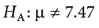
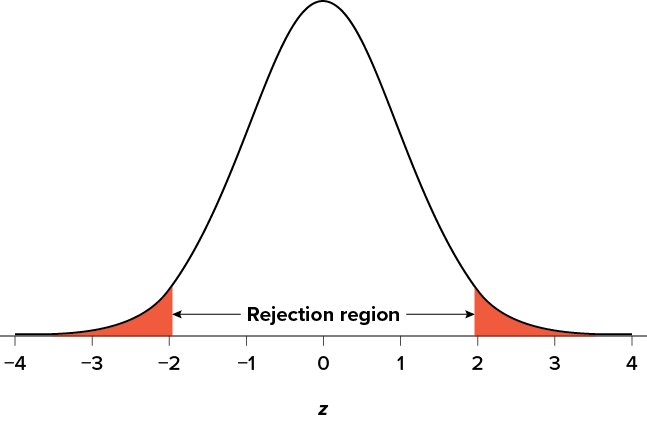
There are two criteria we use to assess whether our data meet the thresholds established by our chosen significance level, and they both have to do with our discussions of probability and distributions. Recall that probability refers to the likelihood of an event, given some situation or set of conditions. In hypothesis testing, that situation is the assumption that the null hypothesis value is the correct value, or that there is no effect. The value laid out in H0 is our condition under which we interpret our results. To reject this assumption, and thereby reject the null hypothesis, we need results that would be very unlikely if the null was true. Now recall that values of z which fall in the tails of the standard normal distribution represent unlikely values. That is, the proportion of the area under the curve as extreme as z—or more extreme than z—is very small as we get into the tails of the distribution. Our significance level corresponds to the area in the tail that is exactly equal to . If we use our normal criterion of a = .05, then 5% of the area under the curve becomes what we call the rejection region (also called the critical region) of the distribution. This is illustrated in Figure 7.1. The shaded rejection region takes us 5% of the area under the curve. Any result that falls in that region is sufficient evidence to reject the null hypothesis.

The rejection region is bounded by a specific z value, as is any area under the curve. In hypothesis testing, the value corresponding to a specific rejection region is called the critical value, zcrit (“z crit”), or z* (hence the other name “critical region”). Finding the critical value works exactly the same as finding the z score corresponding to any area under the curve as we did in Unit 1. If we go to the normal table, we will find that the z score corresponding to 5% of the area under the curve is equal to 1.645 (z = 1.64 corresponds to .0505 and z = 1.65 corresponds to .0495, so .05 is exactly in between them) if we go to the right and −1.645 if we go to the left. The direction must be determined by your alternative hypothesis, and drawing and shading the distribution is helpful for keeping directionality straight.

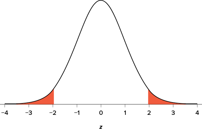
Suppose, however, that we want to do a non-directional test. We need to put the critical region in both tails, but we don’t want to increase the overall size of the rejection region (for reasons we will see later). To do this, we simply split it in half so that an equal proportion of the area under the curve falls in each tail’s rejection region. For a = .05, this means 2.5% of the area is in each tail, which, based on the z table, corresponds to critical values of z* = ±1.96. This is shown in Figure 7.2.

Thus, any z score falling outside ±1.96 (greater than 1.96 in absolute value) falls in the rejection region. When we use z scores in this way, the obtained value of z (sometimes called z obtained and abbreviated zobt) is something known as a test statistic, which is simply an inferential statistic used to test a null hypothesis. The formula for our z statistic has not changed:

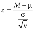
To formally test our hypothesis, we compare our obtained z statistic to our critical z value. If zobt > zcrit, that means it falls in the rejection region (to see why, draw a line for z = 2.5 on Figure 7.1 or Figure 7.2) and so we reject H0. If zobt < zcrit, we fail to reject. Remember that as z gets larger, the corresponding area under the curve beyond z gets smaller. Thus, the proportion, or p value, will be smaller than the area for , and if the area is smaller, the probability gets smaller. Specifically, the probability of obtaining that result, or a more extreme result, under the condition that the null hypothesis is true gets smaller.

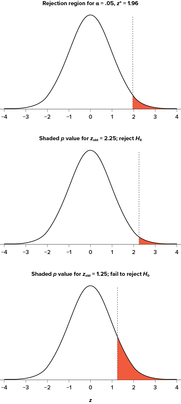
The z statistic is very useful when we are doing our calculations by hand. However, when we use computer software, it will report to us a p value, which is simply the proportion of the area under the curve in the tails beyond our obtained z statistic. We can directly compare this p value to to test our null hypothesis: if p < a, we reject H0, but if p > a, we fail to reject. Note also that the reverse is always true. If we use critical values to test our hypothesis, we will always know if p is greater than or less than . If we reject, we know that p < a because the obtained z statistic falls farther out into the tail than the critical z value that corresponds to , so the proportion (p value) for that z statistic will be smaller. Conversely, if we fail to reject, we know that the proportion will be larger than because the z statistic will not be as far into the tail. This is illustrated for a one-tailed test in Figure 7.3.

When the null hypothesis is rejected, the effect is said to have statistical significance, or be statistically significant. For example, in the Physicians’ Reactions case study, the probability value is .0057. Therefore, the effect of obesity is statistically significant and the null hypothesis that obesity makes no difference is rejected. It is important to keep in mind that statistical significance means only that the null hypothesis of exactly no effect is rejected; it does not mean that the effect is important, which is what “significant” usually means. When an effect is significant, you can have confidence the effect is not exactly zero. Finding that an effect is significant does not tell you about how large or important the effect is.

Do not confuse statistical significance with practical significance. A small effect can be highly significant if the sample size is large enough.

Why does the word “significant” in the phrase “statistically significant” mean something so different from other uses of the word? Interestingly, this is because the meaning of “significant” in everyday language has changed. It turns out that when the procedures for hypothesis testing were developed, something was “significant” if it signified something. Thus, finding that an effect is statistically significant signifies that the effect is real and not due to chance. Over the years, the meaning of “significant” changed, leading to the potential misinterpretation.

The Hypothesis Testing Process

A Four-Step Procedure

The process of testing hypotheses follows a simple four-step procedure. This process will be what we use for the remainder of the textbook and course, and although the hypothesis and statistics we use will change, this process will not.

Step 1: State the Hypotheses

Your hypotheses are the first thing you need to lay out. Otherwise, there is nothing to test! You have to state the null hypothesis (which is what we test) and the alternative hypothesis (which is what we expect). These should be stated mathematically as they were presented above and in words, explaining in normal English what each one means in terms of the research question.

The obesity example null hypothesis in English would be

Ho:There is no difference the time spent with obesity patients compared to time spent with average patients.

The alternative hypothesis in English would be:

Ha: There is a difference between the time spent with obese patients compared with average patients.

Step 2: Find the Critical Values

Next, we formally lay out the criteria we will use to test our hypotheses. There are two pieces of information that inform our critical values: , which determines how much of the area under the curve composes our rejection region, and the directionality of the test, which determines where the region will be.

Step 3: Calculate the Test Statistic

Once we have our hypotheses and the standards we use to test them, we can collect data and calculate our test statistic—in this case z. This step is where the vast majority of differences in future chapters will arise: different tests used for different data are calculated in different ways, but the way we use and interpret them remains the same.

Step 4: Make the Decision

Finally, once we have our obtained test statistic, we can compare it to our critical value and decide whether we should reject or fail to reject the null hypothesis. When we do this, we must interpret the decision in relation to our research question, stating what we concluded, what we based our conclusion on, and the specific statistics we obtained.

Example Interview Callbacks

Let’s see how hypothesis testing works in action by working through an example. Here is an example comparing a sample mean to a population mean. Say you want to look at the number of interview callbacks for recent college graduates based on ethnicity.  The known population mean for interview callbacks is = 8.00 and the known population standard deviation is s = 0.50.  You survey 25 college graduates who are Black and find that, on average, they receive 7.75 callbacks.  This scenario has all of the information we need to begin our hypothesis testing procedure.

Step 1: State the Hypotheses

We will need both a null and an alternative hypothesis written both mathematically and in words. We’ll always start with the null hypothesis:

EXAMPLE:

H _O:  There is no difference in the number of callbacks between the sample of Black graduates and the general population of graduates.

Our assumption of no difference, the null hypothesis, is that this mean is exactly the same as the known population mean value we want it to match, 8.00. Now let’s do the alternative:

H_A: There is a difference in the number of callbacks between the sample of Black graduates and the general population of graduates.

In this case, we don’t know if the number of callbacks is more or less, so we do a two-tailed alternative hypothesis that there is a difference.

Step 2: Find the Critical Values

Our critical values are based on two things: the directionality of the test and the level of significance. We decided in Step 1 that a two-tailed test is the appropriate directionality. We were given no information about the level of significance, so we assume that a = .05 is what we will use. As stated earlier in the chapter, the critical values for a two-tailed z test at a = .05 are z* = ±1.96. This will be the criteria we use to test our hypothesis. We can now draw out our distribution, as shown in Figure 7.4, so we can visualize the rejection region and make sure it makes sense.

Step 3: Calculate the Test Statistic and Effect Size

Now we come to our formal calculations. Let’s say that we collect data and finds that the average amount of callbacks for Black graduates M = 7.75 callbacks. We can now plug this value, along with the values presented in the original problem, into our equation for z:

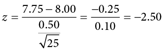
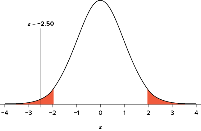
So our test statistic is z = −2.50, which we can draw onto our rejection region distribution as shown in Figure 7.5.

Step 4: Make the Decision

Looking at Figure 7.5, we can see that our obtained z statistic falls in the rejection region. We can also directly compare it to our critical value: in terms of absolute value, −2.50 > −1.96, so we reject the null hypothesis. We can now write our conclusion:

Reject H0. Based on the sample of 25 Black graduates, we can conclude they receive fewer callbacks (M = 7.75 cups) than callbacks received in the general population., z = −2.50, p < .05

When we write our conclusion, we write out the words to communicate what it actually means, but we also include the average number of callbacks for the population , the z statistic and p value. We don’t know the exact p value, but we do know that because we rejected the null, it must be less than  .05.

Social Justice Example:
In an employment discrimination case, if our test statistic falls in the rejection region, we conclude there is strong evidence that hiring practices are not equal. This doesn’t prove discrimination in an absolute sense, but it provides statistical evidence that the null (no difference) is unlikely to be true. Courts and policymakers often rely on this type of statistical reasoning.

Other Considerations in Hypothesis Testing

There are several other considerations we need to keep in mind when performing hypothesis testing.

Errors in Hypothesis Testing

In the Physicians’ Reactions case study, the probability value associated with the significance test is .0057. Therefore, the null hypothesis was rejected, and it was concluded that physicians intend to spend less time with obese patients. Despite the low probability value, it is possible that the null hypothesis of no true difference between obese and average-weight patients is true and that the large difference between sample means occurred by chance. If this is the case, then the conclusion that physicians intend to spend less time with obese patients is in error. This type of error is called a Type I error. More generally, a Type I error occurs when a significance test results in the rejection of a true null hypothesis.

By one common convention, if the probability value is below .05, then the null hypothesis is rejected. Another convention, although slightly less common, is to reject the null hypothesis if the probability value is below .01. The threshold for rejecting the null hypothesis is called the level or simply . It is also called the significance level. As discussed in the introduction to hypothesis testing, it is better to interpret the probability value as an indication of the weight of evidence against the null hypothesis than as part of a decision rule for making a reject or do-not-reject decision. Therefore, keep in mind that rejecting the null hypothesis is not an all-or-nothing decision.

The Type I error rate is affected by the level: the lower the level the lower the Type I error rate. It might seem that is the probability of a Type I error. However, this is not correct. Instead, is the probability of a Type I error given that the null hypothesis is true. If the null hypothesis is false, then it is impossible to make a Type I error.

The second type of error that can be made in significance testing is failing to reject a false null hypothesis. This kind of error is called a Type II error. Unlike a Type I error, a Type II error is not really an error. When a statistical test is not significant, it means that the data do not provide strong evidence that the null hypothesis is false. Lack of significance does not support the conclusion that the null hypothesis is true. Therefore, a researcher should not make the mistake of incorrectly concluding that the null hypothesis is true when a statistical test was not significant. Instead, the researcher should consider the test inconclusive. Contrast this with a Type I error in which the researcher erroneously concludes that the null hypothesis is false when, in fact, it is true.

A Type II error can only occur if the null hypothesis is false. If the null hypothesis is false, then the probability of a Type II error is called b (“beta”). The probability of correctly rejecting a false null hypothesis equals 1 − b and is called statistical power. Power is simply our ability to correctly detect an effect that exists. It is influenced by the size of the effect (larger effects are easier to detect), the significance level we set (making it easier to reject the null makes it easier to detect an effect, but increases the likelihood of a Type I error), and the sample size used (larger samples make it easier to reject the null).

Example:
In social justice work, Type I and Type II errors both carry important consequences. A Type I error might mean wrongly concluding there is discrimination where none exists, potentially damaging credibility. A Type II error might mean failing to detect real discrimination, allowing injustice to persist. Researchers must balance these risks — lowering alpha reduces false positives but raises the risk of missing real inequities. This is why sample size and study design are so important when researching marginalized groups, where smaller numbers can make effects harder to detect.

Hypothesis Testing and Equity
Hypothesis testing provides a framework for asking whether inequalities we observe are due to chance or reflect deeper systemic patterns. By carefully defining null and alternative hypotheses, setting thresholds, and interpreting results, we can turn observations into evidence. For social justice, this is critical: it equips us to say with confidence when disparities are not random but patterned and persistent. Hypothesis testing therefore gives us a scientific foundation for challenging inequities and advocating for meaningful change.

Exercises

1. In your own words, explain what the null hypothesis is.
2. What are Type I and Type II errors?
3. What is ?
4. Why do we phrase null and alternative hypotheses with population parameters and not sample means?
5. If our null hypothesis is “H0 : = 40,” what are the three possible alternative hypotheses?
6. Determine whether you would reject or fail to reject the null hypothesis in the following situations:
   1. z = 1.99, two-tailed test at a = .05
   2. z = 0.34, z* = 1.645
   3. p = .03, a = .05
   4. p = .015, a = .01
7. You are part of a trivia team and have tracked your team’s performance since you started playing, so you know that your scores are normally distributed with = 78 and s = 12. Recently, a new person joined the team, and you think the scores have gotten better. Use hypothesis testing to see if the average score has improved based on 9 weeks’ worth of score data where is 88.75.
8. You get hired as a server at a local restaurant, and the manager tells you that servers’ tips are $42 on average but vary about $12 ( = 42, s = 12). You decide to track your tips to see if you make a different amount, but because this is your first job as a server, you don’t know if you will make more or less in tips. After working 16 shifts, you find that your average nightly amount is $44.50 from tips. Test for a difference between this value and the population mean at the a = .05 level of significance.