
1 Chapter 1: Introduction
This chapter provides an overview of statistics as a field of study and presents terminology that will be used throughout the course.
What Are Statistics?
Statistics include numerical facts and figures that help us understand patterns in society. For instance:
- Black Americans are incarcerated at more than five times the rate of white Americans.
- Women in the United States earn, on average, 82 cents for every dollar earned by men.
- Nearly 1 in 5 transgender people in the U.S. has experienced homelessness.
- By the year 2050, climate change could displace over 200 million people worldwide.
The study of statistics involves mathematics and relies on numerical calculations. However, it also heavily depends on how data is collected and how statistics are interpreted. Consider the following three examples where the numbers might be correct, but the conclusions drawn from them are misleading. Try to identify the major flaw in each interpretation before reading the explanation.
-
A city passes a new law restricting unhoused individuals from sleeping in public spaces. A year later, official reports show a 40% decrease in visible homelessness. Thus, the law successfully reduced homelessness.
- Major flaw: A reduction in visible homelessness does not necessarily mean fewer people are unhoused. Instead, the law may have pushed people into less visible areas, such as encampments in wooded areas or abandoned buildings. This is an example of a measurement issue—what is being counted does not necessarily reflect reality.
-
Cities with more social justice protests also have higher crime rates. Thus, protests cause crime.
- Major flaw: The presence of both protests and higher crime rates can often be explained by other factors, such as systemic inequality, police responses, or urban density. This is an example of the third-variable problem, where two factors appear related but are actually influenced by another variable.
-
The percentage of women in leadership positions in Fortune 500 companies has doubled over the past decade. Thus, gender inequality in the workplace has been solved.
- Major flaw: While the percentage may have increased, the actual number might still be quite low. If only 3% of CEOs were women a decade ago and now it is 6%, that is still a significant disparity. Additionally, this statistic does not address other forms of workplace inequality, such as pay gaps, hiring discrimination, or lack of parental leave policies.
These examples illustrate that statistics are not just numbers; they are shaped by how they are collected, interpreted, and presented. In the broadest sense, “statistics” refers to a range of techniques and procedures for analyzing, interpreting, displaying, and making decisions based on data.
Statistics is the language of social science and activism. Understanding and communicating with statistics enables researchers, policymakers, and activists to articulate their findings, challenge misconceptions, and advocate for meaningful social change. It is an objective, precise, and powerful tool for advancing justice and equity in society.
What a Statistics Course Is Not
Many sociology students dread the idea of taking a statistics course, and more than a few have changed majors upon learning that it is a requirement. That is because many students view statistics as a math class, which is actually not true. While many of you will not believe this or agree with it, statistics isn’t math.
Although math is a central component of it, statistics is a broader way of organizing, interpreting, and communicating information in an objective manner. Indeed, great care has been taken to eliminate as much math from this course as possible (students who do not believe this are welcome to ask the professor what matrix algebra is). Statistics is a way of viewing reality as it exists around us in a way that we otherwise could not.
Why Do We Study Statistics?
Virtually every student of the behavioral sciences takes some form of statistics class. This is because statistics is how we communicate in science. It serves as the link between a research idea and usable conclusions. Without statistics, we would be unable to interpret the massive amounts of information contained in data. Even small datasets contain hundreds—if not thousands—of numbers, each representing a specific observation we made. Without a way to organize these numbers into a more interpretable form, we would be lost, having wasted the time and money of our participants, ourselves, and the communities we serve.
Beyond its use in science, however, there is a more personal reason to study statistics. Like most people, you probably feel that it is important to “take control of your life.” But what does this mean? Partly, it means being able to properly evaluate the data and claims that bombard you every day. If you cannot distinguish good from faulty reasoning, then you are vulnerable to manipulation and to decisions that are not in your best interest. Statistics provides tools that you need in order to react intelligently to information you hear or read. In this sense, statistics is one of the most important things that you can study.
To be more specific, here are some claims that we have heard on several occasions. (We are not saying that each one of these claims is true!)
-
Nearly 40% of unhoused individuals in the U.S. are Black, even though Black people make up only about 13% of the population.
-
Latinx workers are twice as likely as white workers to earn less than $15 per hour.
-
Transgender people are more than four times as likely to experience violent victimization compared to cisgender people.
-
About 1 in 5 women report experiencing sexual harassment in the workplace each year.
-
Only 5% of Fortune 500 CEOs are women, and less than 2% are women of color.
-
Indigenous people in the U.S. are incarcerated at a rate 38% higher than the national average.
-
A recent study shows that students from low-income families are nearly 30% less likely to graduate college within six years compared to wealthier peers.
-
Black women are three times more likely to die from pregnancy-related causes than white women.
-
There’s about a 50% chance that in a group of 23 people, at least two share the same birthday — a classic stats paradox that surprises many students.
All of these claims are statistical in character. We suspect that some of them sound familiar; if not, we bet that you have heard other claims like them. Notice how diverse the examples are. They come from psychology, health, law, sports, business, etc. Indeed, data and data interpretation show up in discourse from virtually every facet of contemporary life.
Statistics are often presented in an effort to add credibility to an argument or advice. You can see this by paying attention to television advertisements. Many of the numbers thrown about in this way do not represent careful statistical analysis. They can be misleading and push you into decisions that you might find cause to regret. For these reasons, learning about statistics is a long step toward taking control of your life. (It is not, of course, the only step needed to do so.) The purpose of this course, beyond preparing you for a career in psychology, is to help you learn statistical essentials. It will make you into an intelligent consumer of statistical claims.
You can take the first step right away. To be an intelligent consumer of statistics, your first reflex must be to question the statistics you encounter. The British Prime Minister Benjamin Disraeli is quoted by Mark Twain as having said, “There are three kinds of lies—lies, damned lies, and statistics.” This quote reminds us why it is so important to understand statistics. So let us invite you to reform your statistical habits from now on. No longer will you blindly accept numbers or findings. Instead, you will begin to think about the numbers, their sources, and most importantly, the procedures used to generate them.
The above section puts an emphasis on defending ourselves against fraudulent claims wrapped up as statistics, but let us look at a more positive note. Just as important as detecting the deceptive use of statistics is the appreciation of the proper use of statistics. You must also learn to recognize statistical evidence that supports a stated conclusion. Statistics are all around you, sometimes used well, sometimes not. We must learn how to distinguish the two cases. In doing so, statistics will likely be the course you use most in your day-to-day life, even if you do not ever run a formal analysis again.
TYPES OF DATA AND HOW TO COLLECT THEM
In order to use statistics, we need data to analyze. Data come in an amazingly diverse range of formats, and each type gives us a unique type of information. In virtually any form, data represent the measured value of variables. In sociology and psychology, we are often interested in people, so we might get a group of people together and measure their levels of stress (one variable), their access to healthcare (a second variable), and their income level (a third variable). Once we have data on these three variables, we can use statistics to understand if and how they are related. Before we do so, we need to understand the nature of our data—what they represent and where they came from.
TYPES OF VARIABLES
When conducting research, experimenters often manipulate variables. For example, an experimenter might compare the effectiveness of four types of tutoring programs. In this case, the variable is “type of program.” When a variable is manipulated by an experimenter, it is called an independent variable. The experiment seeks to determine the effect of the independent variable on student performance. In this example, academic achievement is called a dependent variable. In general, the independent variable is manipulated by the experimenter, and its effects on the dependent variable are measured.
Example #1: Does raising the minimum wage reduce stress?
Researchers could compare three groups of workers: those earning below $15/hour, those earning exactly $15/hour, and those earning above $20/hour. After six months, surveys and health measures could be used to assess stress levels.
-
Independent variable: wage level (below $15, $15, above $20)
-
Dependent variable: measured stress levels
Example #2: Do police body cameras reduce use-of-force incidents?
In a study of police departments, some officers are randomly assigned to wear body cameras while others are not. Researchers track the number of force-related complaints filed by community members over a year.
-
Independent variable: body camera use (yes or no)
-
Dependent variable: number of use-of-force complaints
Example #3: Does providing free school breakfast improve academic outcomes?
A school district implements a free breakfast program in some schools but not others. After a year, researchers compare standardized test scores between the two groups.
-
Independent variable: breakfast program (provided vs. not provided)
-
Dependent variable: test scores
LEVELS OF AN INDEPENDENT VARIABLE
If an experiment compares an experimental treatment with a control treatment, then the independent variable (type of treatment) has two levels: experimental and control. If an experiment were comparing five types of health insurance coverage, then the independent variable (type of coverage) would have 5 levels. In general, the number of levels of an independent variable is the number of experimental conditions.
Qualitative and Quantitative Variables
An important distinction between variables is between qualitative variables and quantitative variables. Qualitative variables are those that express a qualitative attribute such as hair color, eye color, religion, favorite movie, gender, and so on. The values of a qualitative variable do not imply a numerical ordering. Values of the variable “religion” differ qualitatively; no ordering of religions is implied. Qualitative variables are sometimes referred to as categorical or nominal variables. Quantitative variables are those variables that are measured in terms of numbers. Some examples of quantitative variables are height, weight, and shoe size.
In the study on the effect of diet discussed previously, the independent variable was type of supplement: none, strawberry, blueberry, and spinach. The variable “type of supplement” is a qualitative variable; there is nothing quantitative about it. In contrast, the dependent variable “memory test” is a quantitative variable since memory performance was measured on a quantitative scale (number correct).
Discrete and Continuous Variables
Variables such as number of children in a household are called discrete variables since the possible scores are discrete points on the scale. For example, a household could have three children or six children, but not 4.53 children. Other variables such as time to respond to a question are continuous variables since the scale is continuous and not made up of discrete steps. The response time could be 1.64 seconds, or it could be 1.64237123922121 seconds. Of course, the practicalities of measurement preclude most measured variables from being truly continuous.
LEVELS OF MEASUREMENT
Before we can conduct a statistical analysis, we need to measure our dependent variable. Exactly how the measurement is carried out depends on the type of variable involved in the analysis. Different types of variables require different methods of measurement. For example, to measure how long it takes someone to complete a job-training program, you might use a calendar or clock. But to measure a community’s sense of safety in their neighborhood, a survey with response options such as “very unsafe,” “somewhat unsafe,” or “very safe” would be more appropriate. And for a variable like racial/ethnic identity, we would simply record the category the respondent selects.
Although the procedures for measurement differ, they can be classified into a few fundamental categories. Each category captures specific properties of data that are important to understand if we want to analyze inequality, evaluate programs, or document disparities accurately. These categories are called scale types (or just scales) and are described in this section.
TYPES OF VARIABLES
When conducting research, experimenters often manipulate variables. For example, an experimenter might compare the effectiveness of different types of community programs. In this case, the variable is “type of program.” When a variable is manipulated by an experimenter, it is called an independent variable. The experiment seeks to determine the effect of the independent variable on outcomes such as health, education, or safety. In this example, the measurable result is called a dependent variable. In general, the independent variable is manipulated by the experimenter, and its effects on the dependent variable are measured.
Example #1: Do school lunch programs improve academic performance?
Researchers study students in schools with free lunch, reduced-price lunch, or no lunch program. After one year, they compare standardized test scores.
-
Independent variable: type of lunch program (free, reduced, none)
-
Dependent variable: academic performance (test scores)
Example #2: Does access to affordable housing reduce health problems?
A study tracks families who receive housing vouchers compared to those who remain on a waiting list. Over five years, researchers measure health outcomes such as rates of asthma and hospital visits.
-
Independent variable: housing status (voucher vs. no voucher)
-
Dependent variable: health outcomes (asthma rates, hospital visits)
Example #3: Do body cameras reduce police use-of-force incidents?
Police departments randomly assign some officers to wear body cameras and others not to. Researchers then record the number of use-of-force complaints filed by community members.
-
Independent variable: body camera use (yes or no)
-
Dependent variable: number of use-of-force complaints
NOMINAL SCALES
When measuring using a nominal scale, one simply names or categorizes responses. Race/ethnicity, gender identity, housing status, and immigration status are examples of variables measured on a nominal scale. The essential point about nominal scales is that they do not imply any ordering among the responses. For example, when classifying people by housing status (housed, unhoused, transitional housing), there is no sense in which “housed” is placed “ahead of” “unhoused.” Responses are merely categories. Nominal scales embody the lowest level of measurement.
ORDINAL SCALES
A researcher wishing to measure students’ sense of belonging on campus might ask them to rate their experiences as “very excluded,” “somewhat excluded,” “somewhat included,” or “very included.” The items in this scale are ordered, ranging from least to most included. This is what distinguishes ordinal from nominal scales. Unlike a nominal scale, an ordinal scale allows a comparison of the degree to which two individuals report belonging. For example, our belonging scale makes it meaningful to assert that one student feels more included than another.
On the other hand, ordinal scales fail to capture important information that will be present in other scales. In particular, the difference between two levels of an ordinal scale cannot be assumed to be the same as the difference between two other levels. In our belonging scale, for example, the difference between “very excluded” and “somewhat excluded” may not be equivalent to the difference between “somewhat included” and “very included.” Nothing in our measurement procedure allows us to determine whether the two differences reflect the same change in belonging. Statisticians express this by saying that the differences between adjacent scale values do not necessarily represent equal intervals on the underlying scale giving rise to the measurements.
Even if we changed the response format to numbers (1 = very excluded, 2 = somewhat excluded, etc.), the meaning would remain ordinal. The jump from 1 to 2 is not guaranteed to be the same as the jump from 3 to 4.
INTERVAL SCALES
An interval scale is a numerical scale in which intervals have the same interpretation throughout. A good example comes from survey research: standardized test scores such as the SAT. The difference between a score of 1000 and 1100 is intended to represent the same difference in performance as the difference between 1200 and 1300.
Interval scales are not perfect, however. They do not have a true zero point even if one of the scaled values happens to carry the name “zero.” For instance, in public opinion polling, “zero” support for a candidate does not literally mean no one supports them — it just reflects the limits of the measurement. Because an interval scale lacks a true zero, it does not make sense to compute ratios. We cannot say that a SAT score of 1200 means a student is “twice as smart” as a student with a score of 600, since the zero point is arbitrary.
RATIO SCALES
The ratio scale of measurement is the most informative scale. It is an interval scale with the additional property that its zero position indicates the absence of the quantity being measured.
An example of a ratio scale is income. A person with $0 income truly has no money, and someone earning $40,000 makes twice as much as someone earning $20,000. This is what makes it a ratio scale: the zero means “none,” and ratios are meaningful.
Another example is hours worked per week. Zero hours means no work at all, while 40 hours is twice as much as 20 hours. Measures such as number of arrests, years of education completed, or distance to the nearest grocery store also fall into the ratio category because they have true zero points.
In practice, researchers often treat interval and ratio data in similar ways because both use numerical values with equal intervals between them. For example, a public opinion survey on immigration policy might use a 1–7 scale of attitudes (interval), while census data could record household income in dollars (ratio). Both can be averaged, graphed, or analyzed using many of the same statistical techniques. The main difference is that ratio data have a true zero point while interval data do not, but for most statistical procedures—like correlation, regression, or ANOVA—the methods apply equally well to both. This is why you will often see interval and ratio data grouped together under the term scale data in statistical software.
What Level of Measurement Is Used for behavioral science Variables?
Rating scales are used frequently in behavioral science research. For example, experimental subjects may be asked to rate their level of pain, how much they like a consumer product, their attitudes about capital punishment, or their confidence in an answer to a test question. Typically these ratings are made on a 5-point or a 7-point scale. These scales are often considered ordinal scales. However, we also treat them as interval scales which makes the assumption that the values are equi-distant. For example, we make the assumption that a treatment that reduces pain from a rated pain level of 3 to a rated pain level of 2 represents the same level of relief as a treatment that reduces pain from a rated pain level of 7 to a rated pain level of 6.
In memory experiments, the dependent variable is often the number of items correctly recalled. What scale of measurement is this? You could reasonably argue that it is a ratio scale. First, there is a true zero point; some subjects may get no items correct at all. Moreover, a difference of one represents a difference of one item recalled across the entire scale. It is certainly valid to say that someone who recalled 12 items recalled twice as many items as someone who recalled only 6 items.
CONSEQUENCES OF LEVEL OF MEASUREMENT
Why are we so interested in the type of scale that measures a dependent variable? The crux of the matter is the relationship between the variable’s level of measurement and the statistics that can be meaningfully computed with that variable. For example, consider a study in which five students are asked to report their housing status, choosing from the categories: housed, temporarily doubled-up, shelter, street, or transitional housing. The researcher codes the results as follows:
| Housing Status | Code |
|---|---|
| Housed | 1 |
| Doubled-up | 2 |
| Shelter | 3 |
| Transitional housing | 4 |
| Street | 5 |
Collecting Data
We are usually interested in understanding a specific group of people. This group is known as the population of interest, or simply the population. The population is the collection of all people who have some characteristic in common; it can be as broad as “all people” if we have a very general research question about human behavior, or it can be extremely narrow, such as “all freshmen psychology majors at Midwestern public universities” if we have a specific group in mind.
POPULATIONS AND SAMPLES
In statistics, we often rely on a sample—that is, a small subset of a larger set of data—to draw inferences about the larger set. The larger set is known as the population from which the sample is drawn.
Example #1: Access to healthcare
Suppose researchers want to know how adults in the United States feel about whether healthcare is affordable. It would not be practical to ask every single adult in the country, so researchers instead survey a smaller group of people. The group of adults surveyed is the sample, while all U.S. adults make up the population.
A sample is typically a small subset of the population. In the case of healthcare attitudes, we might sample a few thousand Americans drawn from the hundreds of millions in the population. But if our sample were made up entirely of people from urban hospitals, it would leave out the experiences of rural residents. Similarly, if the sample included only people with private insurance, it would fail to represent those on Medicaid or those who are uninsured. This is the problem of sampling bias: when our sample over-represents one kind of person, our results cannot be generalized to the full population.
Example #2: College affordability
Imagine we are interested in how many jobs college students are working, on average, while pursuing their degrees. The population in this case is all U.S. college students. Because there are millions of students enrolled in thousands of institutions, it would be impossible to collect work-hour data from everyone. Instead, we select a sample of students from a mix of public and private colleges, community colleges, and universities. If we found in our sample that students work an average of 20 hours per week, we might infer that this is close to the true population average. But we must be cautious: if our sample leaned heavily toward community colleges (where students are more likely to work longer hours), then the estimate might overstate the work hours of all college students. Again, unrepresentative samples can mislead.
To solidify your understanding of sampling bias, consider the following examples. Identify the population and the sample, and then ask whether the sample is likely to give accurate information.
Example #3: School climate survey
A high school principal wants to know how safe students feel on campus. She distributes surveys, but only to students in the honors program. From their responses, she concludes that students generally feel safe.
-
Population: all students in the high school
-
Sample: honors program students
-
Problem: honors students may have different experiences of school climate than students in other tracks, so the sample is not representative.
Example #4: Housing insecurity on campus
A researcher wants to estimate how many students at a university have experienced housing insecurity. She asks for volunteers and receives responses from 30 students. She reports that 90% of students have struggled with housing.
-
Population: all students at the university
-
Sample: 30 volunteers
-
Problem: students experiencing housing insecurity are more likely to volunteer, so the estimate may exaggerate the true prevalence.
Simple Random Sampling
Researchers adopt a variety of sampling strategies. The most straightforward is simple random sampling. Such sampling requires every member of the population to have an equal chance of being selected into the sample. In addition, the selection of one member must be independent of the selection of every other member. That is, picking one member from the population must not increase or decrease the probability of picking any other member (relative to the others). In this sense, we can say that simple random sampling chooses a sample by pure chance. To check your understanding of simple random sampling, consider the following example. What is the population? What is the sample? Was the sample picked by simple random sampling? Is it biased?
Example #5: A research scientist is interested in studying the experiences of twins raised together versus those raised apart. She obtains a list of twins from the National Twin Registry, and selects two subsets of individuals for her study. First, she chooses all those in the registry whose last name begins with Z. Then she turns to all those whose last name begins with B. Because there are so many names that start with B, however, our researcher decides to incorporate only every other name into her sample. Finally, she mails out a survey and compares characteristics of twins raised apart versus together.
In Example #5, the population consists of all twins recorded in the National Twin Registry. It is important that the researcher only make statistical generalizations to the twins on this list, not to all twins in the nation or world. That is, the National Twin Registry may not be representative of all twins. Even if inferences are limited to the Registry, a number of problems affect the sampling procedure we described. For instance, choosing only twins whose last names begin with Z does not give every individual an equal chance of being selected into the sample. Moreover, such a procedure risks over-representing ethnic groups with many surnames that begin with Z. There are other reasons why choosing just the Zs may bias the sample.
Perhaps such people are more patient than average because they often find themselves at the end of the line! The same problem occurs with choosing twins whose last name begins with B. An additional problem for the Bs is that the every-other-one procedure disallowed adjacent names on the B part of the list from being both selected. Just this defect alone means the sample was not formed through simple random sampling.
Sample Size Matters
Recall that the definition of a random sample is a sample in which every member of the population has an equal chance of being selected. This means that the sampling procedure rather than the results of the procedure define what it means for a sample to be random. Random samples, especially if the sample size is small, are not necessarily representative of the entire population. For example, if a random sample of 20 subjects were taken from a population with an equal number of males and females, there would be a nontrivial probability (.06) that 70% or more of the sample would be female. Such a sample would not be representative, although it would be drawn randomly. Only a large sample size makes it likely that our sample is close to representative of the population. For this reason, inferential statistics take into account the sample size when generalizing results from samples to populations. In later chapters, you’ll see what kinds of mathematical techniques ensure this sensitivity to sample size.
More Complex Sampling
Sometimes it is not feasible to build a sample using simple random sampling. To see the problem, consider the fact that both Dallas and Houston competed to be hosts of the 2012 Olympics. Imagine that you had been hired to assess whether most Texans preferred Houston to Dallas as the host, or the reverse. Given the impracticality of obtaining the opinion of every single Texan, you had to construct a sample of the Texas population. But notice how difficult it would have been to proceed by simple random sampling. For example, how would you have contacted those individuals who didn’t vote and didn’t have a phone? Even among people you found in the telephone book, how could you have identified those who had just relocated to another state (and had no reason to inform you of their move)? What would you have done about the fact that since the beginning of the study, an additional 4,212 people took up residence in the state of Texas? As you can see, it is sometimes very difficult to develop a truly random procedure. For this reason, other kinds of sampling techniques have been devised. We now discuss two of them.
Stratified Sampling
Since simple random sampling often does not ensure a representative sample, a sampling method called stratified random sampling is sometimes used to make the sample more representative of the population. This method can be used if the population has a number of distinct “strata” or groups. In stratified sampling, you first identify members of your sample who belong to each group. Then you randomly sample from each of those subgroups in such a way that the sizes of the subgroups in the sample are proportional to their sizes in the population.
Let’s take an example: Suppose you were interested in views of capital punishment at an urban university. You have the time and resources to interview 200 students. The student body is diverse with respect to age; many older people work during the day and enroll in night courses (average age is 39), while younger students generally enroll in day classes (average age of 19). It is possible that night students have different views about capital punishment than day students. If 70% of the students were day students, it makes sense to ensure that 70% of the sample consisted of day students. Thus, your sample of 200 students would consist of 140 day students and 60 night students. The proportion of day students in the sample and in the population (the entire university) would be the same. Inferences to the entire population of students at the university would therefore be more secure.
Convenience Sampling
Not all sampling methods are perfect, and sometimes that’s okay. For example, if we are beginning research into a completely unstudied area, we may sometimes take some shortcuts to quickly gather data and get a general idea of how things work before fully investing a lot of time and money into well-designed research projects with proper sampling. This is known as convenience sampling, named for its ease of use. In limited cases, such as the one just described, convenience sampling is okay because we intend to follow up with a representative sample. Unfortunately, sometimes convenience sampling is used due only to its convenience without the intent of improving on it in future work.
Types of Statistical Analyses
Now that we understand the nature of our data, let’s turn to the types of statistics we can use to interpret them. There are two types of statistics: descriptive and inferential.
Descriptive Statistics
Descriptive statistics are numbers that are used to summarize and describe data. The word “data” refers to the information that has been collected from an experiment, a survey, a historical record, etc. (By the way, data is plural. One piece of information is called a datum.) If we are analyzing birth certificates, for example, a descriptive statistic might be the percentage of certificates issued in New York State, or the average age of the mother. Any other number we choose to compute also counts as a descriptive statistic for the data from which the statistic is computed. Several descriptive statistics are often used at one time to give a full picture of the data.
Descriptive statistics are just descriptive. They do not involve generalizing beyond the data at hand. Generalizing from our data to another set of cases is the business of inferential statistics, which you’ll be studying in another section. Here we focus on (mere) descriptive statistics.
Some descriptive statistics are shown in Table 1.1. The table shows the average salaries for various occupations in the United States in 1999. Descriptive statistics like these offer insight into American society. It is interesting to note, for example, that we pay the people who educate our children and who protect our citizens a great deal less than we pay people who take care of our feet or our teeth.
Table 1.1. Average salaries for various U.S. occupations in 1999.
|
Occupation |
Salary |
|---|---|
|
Pediatricians |
$112,760 |
|
Dentists |
$106,130 |
|
Podiatrists |
$100,090 |
|
Physicists |
$76,140 |
|
Architects |
$53,410 |
|
School, clinical, and counseling psychologists |
$49,720 |
|
Flight attendants |
$47,910 |
|
Elementary school teachers |
$39,560 |
|
Police officers |
$38,710 |
|
Floral designers |
$18,980 |
For more descriptive statistics, consider Table 1.2. It shows the number of unmarried men per 100 unmarried women in U.S. metro areas in 1990. From this table we see that men outnumber women most in Jacksonville, North Carolina, and women outnumber men most in Sarasota, Florida. You can see that descriptive statistics can be useful if we are looking for an opposite-sex partner! (These data come from the Information Please Almanac.)
Table 1.2. Number of unmarried men per 100 unmarried women in U.S. metro areas in 1990. note: Unmarried includes never–married, widowed, and divorced persons, 15 years or older.
|
Cities with Mostly Men |
Men per 100 Women |
Cities with Mostly Women |
Men per 100 Women |
|
1. Jacksonville, North Carolina |
224 |
1. Sarasota, Florida |
66 |
|---|---|---|---|
|
2. Killeen–Temple, Texas |
123 |
2. Bradenton, Florida |
68 |
|
3. Fayetteville, North Carolina |
118 |
3. Altoona, Pennsylvania |
69 |
|
4. Brazoria, Texas |
117 |
4. Springfield, Illinois |
70 |
|
5. Lawton, Oklahoma |
116 |
5. Jacksonville, Tennessee |
70 |
|
6. State College, Pennsylvania |
113 |
6. Gadsden, Alabama |
70 |
|
7. Clarksville–Hopkinsville, Tennessee–Kentucky |
113 |
7. Wheeling, West Virginia–Ohio |
70 |
|
8. Anchorage, Alaska |
112 |
8. Charleston, West Virginia |
71 |
|
9. Salinas–Seaside–Monterey, California |
112 |
9. St. Joseph, Missouri |
71 |
|
10. Bryan–College Station, Texas |
111 |
10. Lynchburg, Virginia |
71 |
These descriptive statistics may make us ponder why the numbers are so disparate in these cities. One potential explanation, for instance, as to why there are more women in Florida than men may involve the fact that elderly individuals tend to move down to the Sarasota region and that women tend to outlive men. Thus, more women might live in Sarasota than men. However, in the absence of proper data, this is only speculation.
There are many descriptive statistics that we can compute from the data in these tables. To gain insight into the improvement in speed over the years, let us divide the men’s times into two pieces, namely, the first 13 races (up to 1952) and the second 13 (starting from 1956). The mean winning time for the first 13 races is 2 hours, 44 minutes, and 22 seconds (written 2:44:22). The mean winning time for the second 13 races is 2:13:18. This is quite a difference (over half an hour). Does this prove that the fastest men are running faster? Or is the difference just due to chance, no more than what often emerges from chance differences in performance from year to year? We can’t answer this question with descriptive statistics alone. All we can affirm is that the two means are “suggestive.”
It is also important to differentiate what we use to describe populations vs. what we use to describe samples. A population is described by a parameter; the parameter is the true value of the descriptive in the population, but one that we can never know for sure. For example, the Bureau of Labor Statistics reports that the average hourly wage of chefs is $23.87. However, even if this number were computed using information from every single chef in the United States (making it a parameter), it would quickly become slightly off as one chef retires and a new chef enters the job market. Additionally, as noted above, there is virtually no way to collect data from every single person in a population. In order to understand a variable, we estimate the population parameter using a sample statistic. Here, the term statistic refers to the specific number we compute from the data (e.g., the average), not the field of statistics. A sample statistic is an estimate of the true population parameter, and if our sample is representative of the population, then the statistic is considered to be a good estimator of the parameter.
Even the best sample will be somewhat off from the full population, earlier referred to as sampling bias, and as a result, there will always be a tiny discrepancy between the parameter and the statistic we use to estimate it. This difference is known as sampling error, and, as we will see throughout the course, understanding sampling error is the key to understanding statistics. Every observation we make about a variable, be it a full research study or observing an individual’s behavior, is incapable of being completely representative of all possibilities for that variable. Knowing where to draw the line between an unusual observation and a true difference is what statistics is all about.
Inferential Statistics
Descriptive statistics are wonderful at telling us what our data look like. However, what we often want to understand is how our data behave. What variables are related to other variables? Under what conditions will the value of a variable change? Are two groups different from each other, and if so, are people within each group different or similar? These are the questions answered by inferential statistics, and inferential statistics are how we generalize from our sample back up to our population. Unit 2 and Unit 3 are all about inferential statistics, the formal analyses and tests we run to make conclusions about our data.
For example, we will learn how to use a t statistic to determine whether people change over time when enrolled in an intervention. We will also use an F statistic to determine if we can predict future values on a variable based on current known values of a variable. There are many types of inferential statistics, each allowing us insight into a different behavior of the data we collect. This course will only touch on a small subset (or a sample) of them, but the principles we learn along the way will make it easier to learn new tests, as most inferential statistics follow the same structure and format.
A Note about Statistical Software
Many pieces of technology support statistical analysis and quantitative data analysis done by psychologists. The statistical software we use is the proprietary Statistical Package for the Social Sciences (SPSS) which can be accessed through the virtual desktop at Palomar College.
Mathematical Notation
As noted earlier, statistics is not math. It does, however, use math as a tool. Many statistical formulas involve summing numbers. Fortunately, there is a convenient notation for expressing summation. This section covers the basics of this summation notation.
Let’s say we have a variable X that represents the weights (in grams) of 4 grapes:
|
Grape |
X |
|---|---|
|
Grape 1 |
4.6 |
|
Grape 2 |
5.1 |
|
Grape 3 |
4.9 |
|
Grape 4 |
4.4 |
The Greek letter  indicates summation.
When all the scores of a variable (such as X) are to be summed, it is often convenient to use the following abbreviated notation:
 = 4.6 + 5.1 + 4.9 + 4.4 equals 19.
Thus it means to sum all the values of X.
Many formulas involve squaring numbers before they are summed. This is indicated as
![]()
Notice that:
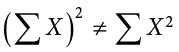
because the expression on the left means to sum up all the values of X and then square the sum ( ), whereas the expression on the right means to square the numbers and then sum the squares (90.54, as shown).
Some formulas involve the sum of cross products. Below are the data for variables X and Y. The cross products (XY) are shown in the third column. The sum of the cross products is  .
.
|
X |
Y |
XY |
|---|---|---|
|
1 |
3 |
3 |
|
2 |
2 |
4 |
|
3 |
7 |
21 |
In summation notation, this is written as:
Exercises
- In your own words, describe why we study statistics.
- For each of the following, determine if the variable is continuous or discrete:
- Time taken to read a book chapter
- Favorite food
- Cognitive ability
- Temperature
- Letter grade received in a class
- For each of the following, determine the level of measurement:
- T-shirt size
- Time taken to run 100-meter race
- First, second, and third place in 100-meter race
- Birthplace
- Temperature in Celsius
- What is the difference between a population and a sample? Which is described by a parameter and which is described by a statistic?
- What is sampling bias? What is sampling error?
- What is the difference between a simple random sample and a stratified random sample?
- What are the two key characteristics of a true experimental design?
- When would we use a quasi-experimental design?
- Use the following dataset for the computations below:
X
Y
2
8
3
8
7
4
5
1
9
4
- What are the most common measures of central tendency and spread?


Answers to Odd-Numbered Exercises
1)
Your answer could take many forms but should include information about objectively interpreting information and/or communicating results and research conclusions.
3)
Ordinal
5)
Ratio
-
- Ordinal
- Nominal
- Interval
7)
Sampling bias is the difference in demographic characteristics between a sample and the population it should represent. Sampling error is the difference between a population parameter and sample statistic that is caused by random chance due to sampling bias.
9)
Random assignment to treatment conditions and manipulation of the independent variable
- 26
- 161
- 109
- 625
The group in an experimental study that is not receiving the treatment being tested.
A variable that exists in indivisible units. For quantitative variables, it is measured in whole numbers that are discrete points on the scale.
Numerical variables that can take on any value in a certain range. Time and distance are continuous; gender, SAT score, and “time rounded to the nearest second” are not.
A subset of a population, often taken for the purpose of statistical inference.
A set of statistics—such as the mean, standard deviation, and skew—that describe a distribution.
The branch of statistics concerned with drawing conclusions about a population from a sample. This is generally done through random sampling, followed by inferences made about central tendency, or any of a number of other aspects of a
