9

So far, we have dealt with data measured on a single variable at a single point in time, allowing us to gain an understanding of the logic and process behind statistics and hypothesis testing. Now, we will look at a slightly different type of data that has new information we couldn’t get at before: change. This is using a within subjects research design, where the same participants are in both samples. For example, one group conducting a pre and post tests. This is a very powerful thing to do, and, as we will see shortly, it involves only a very slight addition to our existing process and does not change the mechanics of hypothesis testing or formulas at all!

Social Justice and Change Over Time
One of the most powerful ways to measure equity and justice is to study change within the same people or communities. Rather than comparing two separate groups, we can look at how the same group experiences outcomes before and after an event, policy, or intervention. For example, we might measure attitudes toward racial equity before and after a workshop, or levels of stress before and after housing support. By linking measurements within individuals, correlated-samples t tests help us see whether meaningful change has occurred, rather than leaving results up to chance.

Change and Differences

Researchers are often interested in change over time. Sometimes we want to see if change occurs naturally, and other times we are hoping for change in response to some manipulation. In each of these cases, we measure a single variable at different times, and what we are looking for is whether or not we get the same score at Time 2 as we did at Time 1. The absolute value of our measurements does not matter—all that matters is the change, or the difference score. Let’s look at an example.

Table 9.1 shows the scores of 5 employees on a survey about their level of ethnic tolerance. The employees were given a survey before and after taking a tolerance workshop to see if the workshop had an impact. The survey was a 1-10 scale in which higher scores represent higher levels of ethnic tolerance. The difference between these scores (i.e., the score after minus the score before) represents improvement in the employees’ tolerance. The third column is what we look at when assessing whether our tolerance workshop was effective. We want to see positive scores, which indicate that the employees’ tolerance level went up. What we are not interested in is how good they were before the training or after the training. Notice that the lowest-scoring employee before the workshop (with a score of 1) improved just as much as the highest scoring employee before the workshop (with a score of 8), regardless of how far apart they were to begin with. There’s also one improvement score of 0, meaning that the workshop did not help this employee. An important factor in this is that the participants received the same assessment at both time points. To calculate improvement or any other difference score, we must measure only a single variable.

When looking at change scores like the ones in Table 9.1, we calculate our difference scores by taking the Time 2 score and subtracting the Time 1 score. That is:

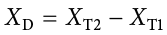
Where XD is the difference score, XT1 is the score on the variable at Time 1, and XT2 is the score on the variable at Time 2. The difference score, XD, will be the data we use to test for improvement or change. We subtract Time 2 minus Time 1 for ease of interpretation; if scores get better, then the difference score will be positive. Similarly, if we’re measuring something like reaction time or depression symptoms that we are trying to reduce, then better outcomes (lower scores) will yield negative difference scores.

In this type of data, what we have are two scores on a single variable. That is, a single observation or data point is comprised of two measurements that are put together into one difference score. This is what makes the analysis of change unique—our ability to link these measurements in a meaningful way.

Example:
Suppose a college launches a mentoring program for first-generation students. We could measure students’ sense of belonging at the start of the semester and again at the end. The difference score (after − before) would tell us whether the program improved students’ sense of inclusion. Here, we aren’t just looking at overall averages — we’re directly measuring change in the same students.

A Rose by Any Other Name . . .

It is important to point out that the correlated samples t test has been called many different things by many different people over the years: related samples, paired samples, matched pairs, repeated measures, dependent measures, dependent samples, and many others. What all of these names have in common is that they describe the analysis of two scores that are related in a systematic way within people or within pairs, which is what each of the datasets usable in this analysis have in common. As such, all of these names are equally appropriate, and the choice of which one to use comes down to preference. In this text, we will refer to correlated samples, though the appearance of any of the other names throughout this chapter should not be taken to refer to a different analysis; they are all the same thing.

Now that we have an understanding of what difference scores are and know how to calculate them, we can use them to test hypotheses. As we will see, this works exactly the same way as testing hypotheses about one sample mean with a t statistic. The only difference is in the format of the null and alternative hypotheses.

Hypotheses of Change and Differences

When we work with difference scores, our research questions have to do with change. Did tolerance levels improve? Did symptoms get better? Did prevalence go up or down? Our hypotheses will reflect this. Remember that the null hypothesis is the idea that there is nothing interesting, notable, or impactful represented in our dataset. In a related samples t test, that takes the form of “no change.” There is no improvement in scores or decrease in symptoms. Thus, our null hypothesis is:

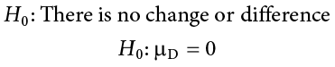
As with our other null hypotheses, we express the null hypothesis for related samples t tests in both words and mathematical notation. The exact wording of the written-out version should be changed to match whatever research question we are addressing (e.g., “There is no change in tolerance scores after workshop”). However, the mathematical version of the null hypothesis is always exactly the same: the average change score is equal to zero. Our population parameter for the average is still , but it now has a subscript D to denote the fact that it is the average change score and not the average raw observation before or after our manipulation. Obviously, individual difference scores can go up or down, but the null hypothesis states that these positive or negative change values are just random chance and that the true average change score across all people is 0.

Our alternative hypotheses will also follow the same format that they did before: they can be directional (one-tailed) if we suspect a change in a specific direction, or we can use an inequality sign to test for any change (two-tailed):

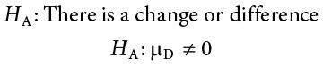
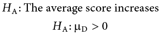
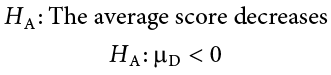
As before, your choice of which alternative hypothesis to use should be specified before you collect data based on your research question and any evidence you might have that would indicate a specific directional (or non-directional) change.

Example:
If we are studying wage equity after a policy change, the null hypothesis might be that average wages for women show no change before and after the policy. The research hypothesis would be that wages improved. This directs our attention not to whether wages are “high” or “low” in absolute terms, but whether progress has been made.

Critical Values and Decision Criteria

As with before, once we have our hypotheses laid out, we need to find the critical values that will serve as our decision criteria. This step has not changed at all from Chapter 8. Our critical values are based on our level of significance (still usually a = .05), the directionality of our test (one-tailed or two-tailed), and the degrees of freedom, which are still calculated as df = number of pairs − 1. Because this is a t test like the last chapter, we will find our critical values on the same t table using the same process of identifying the correct column based on our significance level and directionality and the correct row based on our degrees of freedom or the next lowest value if our exact degrees of freedom are not presented. After we calculate our test statistic, our decision criteria are the same as well: p < a or tobt > t*.

Example:
Imagine evaluating the effect of bail reform on court appearance rates. If the same individuals are tracked before and after reform, the null would say there is no change in appearance rates. If our correlated-samples t statistic falls into the rejection region, we would conclude the reform meaningfully changed outcomes — moving beyond anecdotes to statistical evidence.

Test Statistic

Our test statistic for our change scores follows exactly the same format as it did for our one-sample t test. In fact, the only difference is in the data that we use. For our change test, we first calculate a difference score as shown above. Then, we use those scores as the raw data in the same mean calculation, standard error formula, and t statistic. Let’s look at each of these.

The mean difference score is calculated in the same way as any other mean: sum each of the individual difference scores and divide by the sample size.

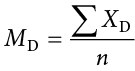
Here we are using the subscript D to keep track of that fact that these are difference scores instead of raw scores; it has no actual effect on our calculation. Using this, we calculate the standard error in the formula below:

Once you calculated the standard error for the difference, our test statistic t is calculated as the Mean difference divided by the standard error. 

As we can see, once we calculate our difference scores from our raw measurements, everything else is exactly the same. Let’s see an example.

Example A: Bad Press

Let’s say that a politician wants to make sure that their new commercial will make them look good to the public, so they recruit 7 people to view the commercial as a focus group. The focus group members fill out a short questionnaire about how they view the politician, then watch the commercial and fill out the same questionnaire a second time. The politician really wants to find significant results, so they test for a change at a = .10. However, they use a two-tailed test since they know that past commercials have not gone over well with the public, and they want to make sure the new one does not backfire. They decide to test their hypothesis using a correlated samples t-tests to see just how spread-out the opinions are.

Step 1: State the Hypotheses

As always, we start with hypotheses:

H₀  :There is no change in how people view the politician.

H₀ : μ_D = 0

H_A  :There is a change in how people view the politician.

H_A : μ_D ≠ 0

Step 2: Find the Critical Values

Just like with our regular hypothesis testing procedure, we will need critical values from the appropriate level of significance and degrees of freedom. Because we have 7 pairs of participants, our degrees of freedom are df = 6. From our t table, we find that the critical value corresponding to this df at this level of significance is t* = 1.943.

Step 3: Calculate the standard error

The data collected before (Time 1) and after (Time 2) the participants viewed the commercial is presented in Table 9.2. In order to calculate our standard error, we will first have to calculate the mean of the difference scores and square them, which are also in Table 9.2. As a reminder, the difference scores are calculated as Time 2 − Time 1.

Complete the chart and use the information to calculate the standard error (σ_diff). The formula should be as follows:

⇒   

Use the standard error (σ_diff) to calculate t:

=

Step 4: Make the Decision

Our calculated t value of 0.46 is less than our critical value of 1.943. Therefore, we failed to reject the null hypothesis.  Fail to reject H0. Based on our focus group of 7 people, we cannot say that the average change in opinion ( = 0.57) was any better or worse after viewing the commercial.

Example:
Sometimes, results show no significant change. For example, a restorative justice program in schools might show little difference in suspension rates before and after implementation in the first year. This doesn’t prove the program “doesn’t work” — it may mean that more time, larger samples, or different measures are needed. In justice research, nonsignificant findings can still guide action by showing us where progress is uneven or slower than expected.

Change, Justice, and Evidence
Correlated-samples t tests allow us to measure change directly, making them especially useful for evaluating programs, policies, and interventions that aim to promote equity. By comparing people to themselves, we can see whether workshops, reforms, or supports truly make a difference. For social justice work, this is invaluable: it helps us separate real progress from chance fluctuations and ensures that claims of improvement are backed by evidence.

Exercises

1. What is the difference between a one-sample t test and a related-samples t test? How are they alike?
2. Name three research questions that could be addressed using a related-samples t test.
3. What are difference scores and why do we calculate them?
4. Why is the null hypothesis for a related-samples t test always D = 0?
5. A researcher is interested in testing whether explaining the processes of statistics helps increase trust in computer algorithms. He wants to test for a difference at the a = .05 level and knows that some people may trust the algorithms less after the training, so he uses a two-tailed test. He gathers pre-post data from 35 people and finds that the average difference score is = 12.10 with a standard deviation of sD = 17.39. Conduct a hypothesis test to answer the research question.
6. Decide whether you would reject or fail to reject the null hypothesis in the following situations:
   1. = 3.50, sD = 1.10, n = 12, a = .05, two-tailed test
   2. t = 2.98, t* = −2.36, one-tailed test to the left
7. Calculate Mean difference scores for the following data:
   

   Time 1	Time 2	XD
   61	83
   75	89
   91	98
   83	92
   74	80
   82	88
   98	98
   82	77
   69	88
   76	79
   91	91
   70	80
   		MD

8. Researchers investigated the extent to which Japanese immigrant mothers encouraged their infants to interact with them or with objects in their environment (such as toys). The researchers observed 8 mothers with their infants. Data are the number of times that mothers encouraged their infants to engage with them or with objects during the observation period. Test the hypothesis at the a = .05 level using the four-step hypothesis testing procedure.
   

   With Mom	With Objects
   15	40
   12	47
   14	32
   10	50
   20	35
   28	45
   12	42
   15	32